VMware Aria Operations for Applications (previously known as Tanzu Observability by Wavefront) supports a join() function that lets you:
- Compare two or more time series and find matches, or, conversely, find the time series that do not match.
- Combine the data points from any matching time series to form a new synthetic time series with point tags from one or both of the input series.
The WQL join() function is modeled after the SQL JOIN operation, which correlates rows of data across 2 or more input tables, and then forms new tables by joining selected portions of the correlated rows. If you are familiar with SQL, then you will recognize many of the WQL join() keywords and concepts.
join() for an inner join is an explicit way to perform series matching between two groups of time series. As an shortcut for certain simple use cases, you can use an operator that performs implicit series matching.Watch Pierre talk about WQL joins and how they’re used. Note that this video was created in 2019 and some of the information in it might have changed. It also uses the 2019 version of the UI.
Time Series as Tables
A WQL join() views time series as tables and then operates on those tables. A time series is a sequence of timestamped points that is identified by a unique combination of metadata:
- A metric name, for example,
cpu.load - A source name, for example,
host-1 - 0 or more point tags (key value pairs), for example,
env=prod dc=Oregon
A join() operation views every time series as a row in a table that has a column for each metadata value. In this model, we use a separate table for each metric name.
Sample Time-Series Tables
Suppose you are running services on several sources, and you want to use a WQL join() to correlate the CPU load with the number of service requests per second on each source. You identify the time series you want to correlate, and refer to them using the ts() expressions ts(cpu.load) and ts(request.rate). Each ts() expression stands for a group of time series with different sources and point-tag values, and you want to use join() to identify any pairs of series that both flow from the same source, and share certain point-tag values.
We represent the time series for each metric as rows in separate tables, which we will use for the various join() examples on this page. The doc uses row indicators like L1 so we can refer to specific time series in later examples. They’re not part of the data!
The first table shows 6 time series that are described by ts(cpu.load). Each series is a unique combination of metric name, source, and values for point tags env and dc:
| Row | metric | source | env= | dc= | Data Points |
|---|---|---|---|---|---|
L1 |
cpu.load | host-1 | prod | Oregon | (timestamp:value, …) |
L2 |
cpu.load | host-2 | dev | Oregon | (timestamp:value, …) |
L3 |
cpu.load | host-3 | prod | Oregon | (timestamp:value, …) |
L4 |
cpu.load | host-1 | prod | NY | (timestamp:value, …) |
L5 |
cpu.load | host-2 | test | NY | (timestamp:value, …) |
L6 |
cpu.load | host-3 | prod | NY | (timestamp:value, …) |
The second table shows 4 time series that are described by ts(request.rate). These series do not have the dc point tag, so the table does not have a column for it. Instead, these series have a service point tag:
| Row | metric | source | env= | service= | Data Points |
|---|---|---|---|---|---|
R1 |
request.rate | host-1 | prod | shopping | (timestamp:value, …) |
R2 |
request.rate | host-2 | dev | shopping | (timestamp:value, …) |
R3 |
request.rate | host-3 | prod | checkout | (timestamp:value, …) |
R4 |
request.rate | host-4 | test | checkout | (timestamp:value, …) |
join() Syntax Overview
Like SQL JOIN, the WQL join() function examines rows from two time-series tables, and determines whether any row from one table correlates with any row from the other. Two rows correlate if they both satisfy a join condition. All join() operations combine the correlated rows into new rows in a new table, and then return a new time series corresponding to each new row. (Some join() types also return time series for the non-correlated rows in one or both tables.)
For example, suppose you want to divide the CPU load by the number of service requests per second on each production, development, or test source. The following join() function accomplishes this by correlating rows from the two tables above:
join(ts(cpu.load) AS ts1 INNER JOIN ts(request.rate) AS ts2 USING(source, env), metric='cpuPerRequest', source=ts1.source, env=ts1.env, ts1 / ts2)
Let’s split out the join() parameters into separate expressions to see what they do:
join(
  ts(cpu.load) AS ts1 INNER JOIN ts(request.rate) AS ts2            <== Join Input and Join Type

  USING(source, env),                                               <== Join Condition
       // ON ts1.source=ts2.source AND ts1.env=ts2.env,             <== alternative syntax

  metric='cpuPerRequest', source=ts1.source, env=ts1.env,           <== Output Metadata

  ts1 / ts2                                                         <== Output Data Expression
  )
For readability, we write the keywords in all caps, but that’s not required.
Join Input and Join Type
ts(cpu.load) AS ts1 INNER JOIN ts(request.rate) AS ts2
- Like SQL
FROM. - ts() expressions specify the time series in a left table (e.g.,
ts(cpu.load)) and a right table (e.g.,ts(request.rate)). - Either or both ts() expressions can include filters, analogous to SQL
WHERE. For example,ts(cpu.load, dc!=Texas) ASassigns an alias to each table (required). For example,ts1is the alias forts(cpu.load).- Do not use reserved words, such as WQL function names, operator names, or SI prefixes. For details, see the rules for valid alias names in Wildcards, Aliases, and Variables.
- Best practice: Make aliases 3 characters or longer.
INNER JOINis one of 4 join types. The join type determines whether and how rows are included in the result table.
Join Condition
USING(source, env), or
ON ts1.source=ts2.source AND ts1.env=ts2.env,
- Syntax alternatives:
USINGorON USINGlists the columns to use when testing for correlated rows:USING(source, env)- Rows satisfy the condition if they share a common value in each listed column. For example, two rows match if they both have
source="host-1"andenv="prod".
- Rows satisfy the condition if they share a common value in each listed column. For example, two rows match if they both have
ONspecifies explicit condition predicates:ON ts1.source=ts2.source AND ts1.env=ts2.env- Predicates use table aliases to qualify column names. For example,
ts1.env=ts2.envcomparesenvvalues from the left table toenvvalues from the right table. - Predicates can include pattern matches, negation, parentheses, and constants. For example,
ON ts1.source!="web*"
- Predicates use table aliases to qualify column names. For example,
Output Metadata
metric='cpuPerRequest', source=ts1.source, env=ts1.env,
- Like SQL
SELECT. - Optional list of expressions that specify the metadata for the result time series. Metadata expressions name the columns in the result table, and assign values to them. For example:
metric=cpuPerRequestspecifies the metric name.env=ts1.envadds a column for a point tag calledenvand assigns it the value ofts1.env.
- Table aliases indicate where point-tag values come from. For example,
ts1.envgetsenvvalues from rows in the left table. - Omitting these expressions introduces a column for a point tag called
_discriminantto differentiate the resulting time series.
Output Data Expression
ts1 / ts2
- Derives the data points for each new time series from the data points of matching input rows.
- Table aliases indicate where the input data points come from. For example,
ts1refers to the data points from a row in the left table.
- Table aliases indicate where the input data points come from. For example,
- Inner joins function as expected only when the output data expression includes both
ts1andts2in some form. - Supports operators
+ - / *and functionsmax(),min(),avg(),median(),sum(),count()to combine data points from both tables. For example:ts1 / ts2divides each value from a left-hand row by the corresponding value from the matching right-hand row.avg(ts1, ts2)averages each value from a left-hand row with the corresponding value from the matching right-hand row.- Values are interpolated if the timestamps do not line up.
- Special syntax
{<alias> | N}specifies the numeric constant to use in place of missing input data points. Required for outer joins. For example,ts1 / {ts2|1}says to divide by1when there is no matching row (and therefore no data points) from the right table.
Join Types
Like SQL JOIN, the WQL join() function supports different types of join operation. Each join type has a different rule for including rows (time series) in the result table.
The following table shows the main types of joins.
- This table shows inclusive joins, which means they include any rows that satisfy the join condition.
- We also support exclusive join types for use cases in which you only want rows that do not satisfy the condition.
| Join Type | Operation |
|---|---|
 |
Include rows from both tables, if they both satisfy a specified join condition. Keywords: JOIN | INNER JOIN |
 |
Include all rows from the left table, and include rows from the right table only if they satisfy a specified join condition. Keywords: LEFT JOIN | LEFT OUTER JOIN |
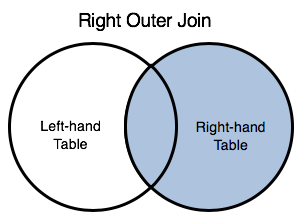 |
Include all rows from the right table, and include rows from left table only if they satisfy a specified join condition. Keywords: RIGHT JOIN | RIGHT OUTER JOIN |
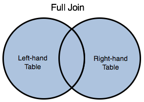 |
Include all rows from both tables, regardless of whether the specified join condition is met or not. Keywords: FULL JOIN | FULL OUTER JOIN |
Inner Join Example
Suppose you have the time series in the tables above, and you want to divide the CPU load by the number of service requests per second on each production, development, or test source. You perform an inner join to identify any pairs of series that both flow from the same source and run in the same environment.
join(
  ts(cpu.load) AS ts1 INNER JOIN ts(request.rate) AS ts2 USING(source, env),
  metric='cpuPerRequest', source=ts1.source, env=ts1.env, service=ts2.service,
  ts1 / ts2
  )
Row Selection
The inner join matches rows (time series) from the left table and right table above, based on the values for the source and env columns. The following table shows the particular rows that match up.
| Row | Left-Hand Series | Inner-Joined With Right-Hand Series | Row |
|---|---|---|---|
| L1 | cpu.load host=host-1 env=prod dc=Oregon |
request.rate host=host-1 env=prod service=shopping |
R1 |
| L2 | cpu.load host=host-2 env=dev dc=Oregon |
request.rate host=host-2 env=dev service=shopping |
R2 |
| L3 | cpu.load host=host-3 env=prod dc=Oregon |
request.rate host=host-3 env=prod service=checkout |
R3 |
| L4 | cpu.load host=host-1 env=prod dc=NY |
request.rate host=host-1 env=prod service=shopping |
R1 |
| L6 | cpu.load host=host-3 env=prod dc=NY |
request.rate host=host-3 env=prod service=checkout |
R3 |
Metadata from Input Rows
Each pair of matching rows in the previous table is the input for a new time series to be returned by the inner join. The following table shows the metadata for each new time series as a separate row, with columns that are specified by the function’s output metadata expressions. For example, row A4 corresponds to a new series that has the metric name cpuPerRequest, source and env values from L4, and the service value from R1.
| New Row | metric | source | env= | service= | Data Points | Input Rows |
|---|---|---|---|---|---|---|
| A1 | cpuPerRequest | host-1 | prod | shopping | Derived from input points | L1, R1 |
| A2 | cpuPerRequest | host-2 | dev | shopping | Derived from input points | L2, R2 |
| A3 | cpuPerRequest | host-3 | prod | checkout | Derived from input points | L3, R3 |
| A4 | cpuPerRequest | host-1 | prod | shopping | Derived from input points | L4, R1 |
| A5 | cpuPerRequest | host-3 | prod | checkout | Derived from input points | L6, R3 |
dc, because the sample join() function did not specify this point tag among its output metadata expressions.Data Derived from Input Rows
The data points of each result series are derived from the data points of the matching input series. In this example, the output data expression ts1 / ts2 says to divide the values of a left-hand series by the values of the matching right-hand series. (For simplicity in this example, we assume that all right-hand values are nonzero.)
The query engine accomplishes this by dividing each value of the left-hand series by the value with the corresponding timestamp from the right-hand series. So, for example, the result series corresponding to row A5 has points that are derived by dividing each value from L6 by the corresponding value from R3.
If the timestamps for the 2 input series do not line up, the query engine interpolates values before combining them.
Left Outer Join Example
Suppose you have the time series in the tables above, and you want to:
- Divide the CPU load by the number of service requests per second on each production, development, or test source.
- See the sources (if any) that are reporting CPU loads, but are not running a monitored service.
You perform a left outer join to return all cpu.load time series, and also to correlate pairs of cpu.load and request.rate series if they flow from the same source and run in the same environment.
join(
  ts(cpu.load) AS ts1 LEFT JOIN ts(request.rate) AS ts2 USING(source, env),
  metric='cpuPerRequest', source=ts1.source, env=ts1.env, service=ts2.service,
  ts1 / {ts2|1}
  )
Row Selection
The left outer join selects all rows (time series) from the left table, plus any row from the right table that matches a left-hand row, based on the values for the source and env columns. The following table shows the selected rows:
| Row | Left-Hand Series | Left-Joined With Right-Hand Series | Row |
|---|---|---|---|
| L1 | cpu.load host=host-1 env=prod dc=Oregon |
request.rate host=host-1 env=prod service=shopping |
R1 |
| L2 | cpu.load host=host-2 env=dev dc=Oregon |
request.rate host=host-2 env=dev service=shopping |
R2 |
| L3 | cpu.load host=host-3 env=prod dc=Oregon |
request.rate host=host-3 env=prod service=checkout |
R3 |
| L4 | cpu.load host=host-1 env=prod dc=NY |
request.rate host=host-1 env=prod service=shopping |
R1 |
| L5 | cpu.load host=host-2 env=test dc=NY |
|
– |
| L6 | cpu.load host=host-3 env=prod dc=NY |
request.rate host=host-3 env=prod service=checkout |
R3 |
Row L5 (a left-hand series) is included in this table, even though it does not match any right-hand series. In contrast, row R4 (a right-hand series) is omitted entirely because it would have no match on the left.
Metadata from Input Rows
The rows in the previous table serve as input for constructing the new time series to be returned by the left outer join. The following table shows the metadata for each new time series as a separate row, with columns that are specified by the function’s output metadata expressions. For example, row B4 corresponds to a new series that has the metric name cpuPerRequest, source and env values from L4, and the service value from R1.
| New Row | metric | source | env= | service= | Data Points | Input Rows |
|---|---|---|---|---|---|---|
| B1 | cpuPerRequest | host-1 | prod | shopping | Derived from input points | L1, R1 |
| B2 | cpuPerRequest | host-2 | dev | shopping | Derived from input points | L2, R2 |
| B3 | cpuPerRequest | host-3 | prod | checkout | Derived from input points | L3, R3 |
| B4 | cpuPerRequest | host-1 | prod | shopping | Derived from input points | L4, R1 |
| B5 | cpuPerRequest | host-2 | test | – | Derived from input points | L5 |
| B6 | cpuPerRequest | host-3 | prod | checkout | Derived from input points | L6, R3 |
From this table, we see that the left outer join returns the same set of time series as the inner join above, plus an additional time series with the metadata given in row B5. This additional series has no service point tag, because there was no right-hand input row to contribute a value for it.
Data Derived from Input Rows
The data points of each new series are derived from the data points of the corresponding input series, as specified by the output data expression.
- When a new series is produced by combining a pair of matching input series, the data points in the new series are derived as for an inner join.
- When a new series (such as B5) is produced from a single left-hand input series, the data points in the new series are derived using the special syntax in the output data expression. The sample output data expression
ts1 / {ts2|1}says to divide the values of a left-hand series by 1 whenever there is no matching right-hand series, as is the case for B5.
You must use the special syntax in a left outer join to provide alternate values for the right-hand series, which might be missing. A result series with missing input values will not display.
You can use the special syntax to provide whatever alternate value makes sense for your use case. In the example, dividing by 1 gives the new series the same data points as the unmatched left-hand input series. In an output expression that uses + to combine data values, however, you can preserve values by specifying 0 as the alternate value, for example, ts1 + {ts2|0}.
Right Outer Join Example
Suppose you have the time series in the tables above, and you want to:
- Divide the CPU load by the number of service requests per second on each production, development, or test source.
- See the services (if any) that are reporting rates, but are not on a source that is also reporting CPU loads.
You perform a right outer join to return all request.rate time series, and also to correlate pairs of request.rate and cpu.load series if they flow from the same source and environment.
join(
  ts(cpu.load) AS ts1 RIGHT JOIN ts(request.rate) AS ts2 USING(source, env),
  metric='cpuPerRequest', source=ts1.source, env=ts1.env, service=ts2.service,
  {ts1|0} / ts2
  )
Row Selection
The right outer join selects all rows (time series) from the right table, plus any row from the left table that matches a right-hand row, based on the values for the source and env columns. The following table shows the selected rows:
| Row | Left-Hand Series | Right-Joined With Right-Hand Series | Row |
|---|---|---|---|
| L1 | cpu.load host=host-1 env=prod dc=Oregon |
request.rate host=host-1 env=prod service=shopping |
R1 |
| L4 | cpu.load host=host-1 env=prod dc=NY |
request.rate host=host-1 env=prod service=shopping |
R1 |
| L2 | cpu.load host=host-2 env=dev dc=Oregon |
request.rate host=host-2 env=dev service=shopping |
R2 |
| L3 | cpu.load host=host-3 env=prod dc=Oregon |
request.rate host=host-3 env=prod service=checkout |
R3 |
| L6 | cpu.load host=host-3 env=prod dc=NY |
request.rate host=host-3 env=prod service=checkout |
R3 |
| – | |
request.rate host=host-4 env=test service=checkout |
R4 |
Row R4 (a right-hand series) is included in this table, even though it does not match any left-hand series. In contrast, row L5 (a left-hand series) is omitted entirely because it would have no match on the right.
Metadata from Input Rows
The rows in the previous table serve as input for constructing the new time series to be returned by the right outer join. The following table shows the metadata for each new time series as a separate row, with columns that are specified by the function’s output metadata expressions. For example, row C5 corresponds to a new series that has the metric name cpuPerRequest, source and env values from L6, and the service value from R3.
| New Row | metric | source | env= | service= | Data Points | Input Rows |
|---|---|---|---|---|---|---|
| C1 | cpuPerRequest | host-1 | prod | shopping | Derived from input points | L1, R1 |
| C2 | cpuPerRequest | host-1 | prod | shopping | Derived from input points | L4, R1 |
| C3 | cpuPerRequest | host-2 | dev | shopping | Derived from input points | L2, R2 |
| C4 | cpuPerRequest | host-3 | prod | checkout | Derived from input points | L3, R3 |
| C5 | cpuPerRequest | host-3 | prod | checkout | Derived from input points | L6, R3 |
| C6 | cpuPerRequest | – | – | checkout | Derived from input points | R4 |
From this table, we see that the right outer join returns the same set of time series as the inner join above, plus an additional time series with the metadata given in row C6. This additional series has no source and env point tag, because there was no left-hand input row to contribute values for them.
Data Derived from Input Rows
The data points of each new series are derived from the data points of the corresponding input series, as specified by the output data expression.
- When a new series is produced by combining a pair of matching input series, the data points in the new series are derived as for an inner join.
- When a new series (such as C6) is produced from a single right-hand input series, the data points in the new series are derived using the special syntax in the output data expression. The sample output data expression
{ts1|0} / ts2says to divide the right-hand series into 0 whenever there is no matching left-hand series, as is the case for C6.
You must use the special syntax in a right outer join to provide alternate values for the left-hand series, which might be missing. A result series with missing input values will not display.
You can use the special syntax to provide whatever alternate value makes sense for your use case. In the example, specifying 0 as the dividend produces a new constant series of 0 for each unmatched right-hand input series.
Exclusive Join Types
You can combine the WQL join() and removeSeries() functions to perform exclusive join operations. An exclusive join starts with an inclusive join type and then filters out any rows (time series) that satisfy the join condition. Exclusive joins are useful for finding hidden issues, as illustrated in our blog on finding silent failures with join().
The following table describes the types of exclusive join.
| Join Type | Operation |
|---|---|
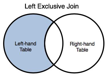 |
Include only rows from the left table that do not satisfy a specified join condition (i.e., that do not match rows of the right table.) join() keywords: LEFT JOIN | LEFT OUTER JOIN Use removeSeries() to filter out matches
|
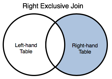 |
Include only rows from the right table that do not satisfy a specified join condition (i.e., that do not match rows of the left table.) join() keywords: RIGHT JOIN | RIGHT OUTER JOIN Use removeSeries() to filter out matches
|
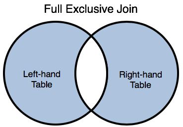 |
Include only the rows from either table that do not satisfy a specified join condition. Use collect() to combine a left outer join and a right outer joinUse removeSeries() to filter out matches
|
Left Exclusive Join Example
Suppose you are running services on various sources, and you know that your services take 3.5 minutes to start up. You can tell that a service has started when it starts reporting metrics, but you’d like to find out if any services have failed to start after 5 minutes.
You can do this by running a left exclusive join between a metric that is reported by the source (e.g., cpu.uptime) and a metric that is reported by the service (e.g., service.uptime), provided that these metrics share common metadata (e.g., an id point tag). You can then investigate any source whose uptime metric does not correspond to a matching service-uptime metric. For example:
removeSeries(
  join(
    ts(cpu.uptime) AS ts1 LEFT JOIN ts(service.uptime) AS ts2 USING(id),
    metric='NeedsAttention', source=ts1.source, env=ts1.env, id=ts1.id, filter-id=ts2.id,
    ts1
    ),
  filter-id="*"
)
In this query, the join() function performs an left outer join that uses the id point tag value as the join condition. Each output series from this function has:
- The specified metric name (
NeedsAttention), - Data values and several metadata values from a
cpu.uptimeseries. - A new
filter-idpoint tag, but only if the join condition has been met:filter-idis added whenever acpu.uptimeseries and aservice.uptimeseries have a matching id.filter-idis not added to an unmatched output series.
The removeSeries() function then filters the results of the join() function by removing any NeedsAttention series that has a filter-id tag. The overall result is a set of time series corresponding to each source that does not have the expected service running on it.