Query Language Tutorial

VMware Aria Operations for Applications (formerly known as Tanzu Observability by Wavefront) includes the Wavefront Query Language (WQL), which lets you retrieve and display data that has been ingested.

• Time series data The query language is particularly well suited to time series data because it accommodates the periodicity, potential irregularity, and streaming nature of that data type.
• Histograms The query language includes functions for manipulating histograms.
• Traces and spans Use the tracing UI to query traces and spans.

This page uses the v2 UI, which allows you to examine your data with chart builder and perform advanced exploration with query editor.

Videos

Watch these videos to get you started. The videos were created between 2017 and 2021 and some of the information in them might have changed. They also use the v1 UI, but the basic workflow remains the same in the v2 UI.

Query Language Basics	Learn about time series metrics, and about how to visualize metrics and filter and group them with Wavefront Query Language. You can also watch the video here .
Intro to Wavefront Query Language	Wavefront Query Language allows you to shape the data you see in your dashboards. The example uses the advanced functions if() at() and corr() to find a problem behavior of a switch in other switches and prevent future problems. You can also watch the video here .
Query Language Advanced Functions	Jason starts by looking at the data format. Then he adds a query to a chart that has only the required metric name. To narrow down the result, he uses a source filter with a wildcard and a point tag filter. You can also watch the video here .

Step 0: What’s a Query?

Before you run your first query, let’s examine a time series and look at the anatomy of a query.

What’s a Time Series?

A time series measures a particular phenomenon over time. In the example below:

• The time series metric is temperature
• Two types are ear and forehead, and the types can show up as values of a location tag.
• You could also associate a source with each time series. In this example, you could have a different time series for each patient.

Anatomy of a Query

Now, let’s look at the anatomy of a query (shown in Chart Builder):

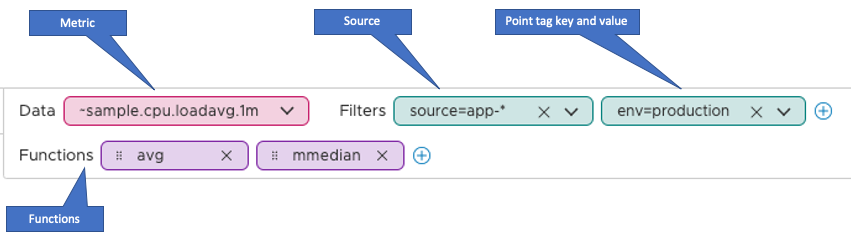
Each query has the following components. Only the metric is required, the other elements are optional, but they help you get the information you’re really interested in.

• A metric (or a constant, such as 10). Above, the metric is temperature. In this example, the metric is ~sample.cpu.loadavg.1m
• One or more sources. Above, sources would have been patients. Here, sources could be the host, VM, container, etc. In this example, the source is app-* – that means metrics that come from db-* are ignored.
• One or more point tags. Above, we have the location point tag - ear and forehead. In this example, we have the env point tag with value production. Only valid point tags can be queried.
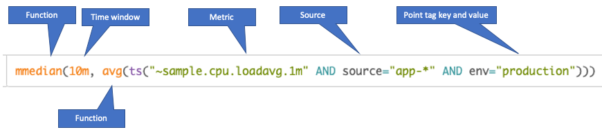
• One or more functions. This example uses the avg() function, and the mmedian() function with a 10-minute time window. The Query Language Reference lists each function with a short description and points to reference pages.

Here’s how the same query looks in the Query Editor.

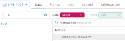
Step 1: Retrieve a Metric

The Chart Builder UI makes it easy to show any metric that’s currently flowing into your product instance. Follow these steps to explore the sample data, included with each product instance.

Log in to your product instance, which has a URL <my_instance>.wavefront.com. Select Dashboards > New Chart. In the Chart Builder, select the metric ~sample.cpu.loadavg.1m. Autocomplete helps with the selection.

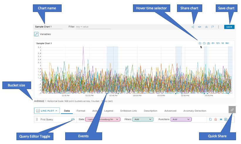
Here’s an annotated screenshot of the first chart you’ll see.

• Chart names are easy to change just by typing.
• For quick zoom in/out, use the hover time selector, which appears when the cursor is on the chart.
• As you zoom in or out, the bucket size (chart resolution) changes.
• Use Share chart or Quick share to share with others.
• Use the Query Editor toggle for some advanced query functionality.
• Notice events that are shown on the time line. These events are often system events associated with alerts, but they can also be user-defined events.
• Make sure that you Save the chart to a new or existing dashboard.

Things to Try

In the chart:

• Use the Hover Time Selector to zoom in and out. You can also select-drag to see part of the chart, then click + or - to return to the default settings.
• Hover over event icons in the Y axis to get details for the event.
• Hover over a time series to see the legend. Press Shift+P to pin the legend.

In Chart Builder:

• Query other ~sample metrics.
• Switch to Query Editor and add a constant (e.g., 100) – but note that you can’t switch back to Chart Builder!

Step 2: Filter by Source and Point Tag

The example chart is quite busy, but we can use filters to focus in.

1. Make sure Data is still ~sample.cpu.loadavg.1m.
2. Click Filters, select source and type app-* to include only time series if the source name starts with app-. This query uses a wildcard character.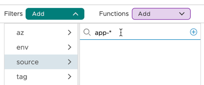
3. Press Enter.
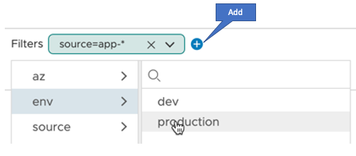
4. Click the Add button and select env > production as the second filter.

Things to Try

• Explore the effect of using different source and point tag filters.
• Add more than one filter for each category, for example, several sources.
• Click the Query Editor toggle </> to see the results in Query Editor.
• Clone the query to experiment more. If you accidentally make a change in the query while you’re in the Query Editor, you can’t return to Chart Builder, so using a clone helps.
• With multiple queries in place, show and hide queries, and drag them to change query order.

Step 3: Apply an Aggregation Function

Aggregation functions allow you to combine points from multiple time series, and to group the results. Let’s take the average first, and then let’s remove the env filter and instead group by environment.

1. Make sure Data is still ~sample.cpu.loadavg.1m.
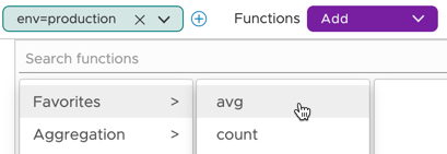
2. Click Functions, and pick Favorites > avg. The result is a single aggregated time series. In Query Editor, this query looks like this: avg(ts(~sample.cpu.loadavg.1m, source="app-*" and env="production"))
3. Remove the `env` filter.
4. Click Functions > Favorites > avg again.
5. Select Group by, then select env, and click Apply. The result is two aggregated time series. You can hover over each line to see which environment it shows. In the Query Editor, you can add the literal , pointTags (you need the comma!), so the query looks like this: avg(ts(~sample.cpu.loadavg.1m, source="app-*"), env, pointTags)
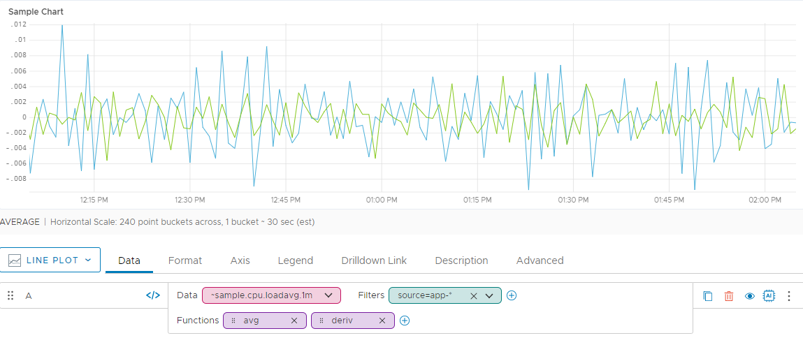
6. Add a second function. For example, you can use the deriv() function to show the rate of change per second for the average. deriv(avg(ts(~sample.cpu.loadavg.1m, source="app-*"), env))

Things to Try

Experiment with some of our other functions, either in Chart Builder or in Query Editor.

• Use one of the Moving Window Time Functions to combine or test the values of a time series over a time sliding window.
• Experiment with Filtering and Comparison Functions. For example, use topk() to return the top numberOfTimeSeries series.

Step 4: See What’s There

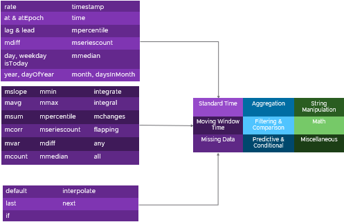
Wavefront Query Language has a rich set of functions for many purposes. The Query Language Reference has the details, here’s an overview (in pictures).

The following diagram shows the main function categories for examining time series metrics. We support additional functions for working with events, histograms, and with traces and spans.

Aggregation, Predictive, and Filtering & Comparison Functions 1. Let’s drill down and look at the first set of functions. The image on the right shows the aggregation, filtering, and predictive functions. The Query Language Reference has the syntax for each function. The function syntax links to a reference page.
Standard Time, Moving Time Window, and Missing Data Functions 2. Next, let's look at a second set of functions. The image on the right shows the standard time, moving window time, and missing data functions. The Query Language Reference has the syntax for each function. The function syntax links to a reference page.
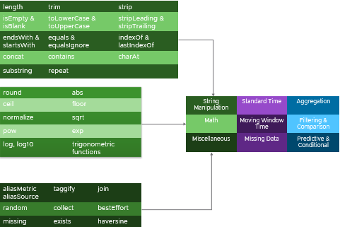
Math, String Manipulation, and Miscellaneous functions 3. Finally, we look at the math, string manipulation, and miscellaneous functions (shown in more detail in the query language reference. The Query Language Reference has the syntax for each function. The function syntax links to a reference page.

Next Steps

What’s next depends on the type of data you’re interested in, and how you want to interact with your data.

Query Types for Different Data

Most users query for time series metrics, but we support interacting with other data.

Charts for metrics also support the following types of queries:

• Events: Query events with events() queries.
• Histograms: Query histograms with hs() queries.
• Traces and spans: Query trace data from the tracing UI with the tracing Query Builder.

Docs, Learning Dashboards, and More!

Our documentation includes tutorials, reference, and guides on the query language. In addition, your product instance includes an Interactive Query Language Explorer dashboard.

• Chart builder can help you come up to speed quickly while using the product.
• If you’re logged in to your product instance, click Integrations on the toolbar and find the Tutorial or the Tour Pro integration. The Tutorial includes an Interactive Query Language Explorer dashboard that shows examples for most functions.
• Wavefront Query Language Reference lists each function and gives query language syntax element. Each function name is a link to a reference page for the function.
• For in-depth discussions and examples, we have a reference page for each function and some Query Language Recipes.

FAQ

This doc set includes videos and explanations from the engineering team that helps you come up to speed quickly:

Question	Doc/Blog	Video
How can I combine multiple series?	Aggregating Time Series	Time Series and Interpolation
Why does my query return NO DATA?	Maybe the time series don’t match. See When Multiple Series Match (Or Not).
I got a warning about pre-aligned data. Why?	To improves performance, the query engine wraps align() around certain functions. See Bucketing with align().
How can I improve query performance?	Consider bucketing with align(). Investigate internal metrics for optimizing performance.