Our Customer Success team has found that customers often want certain information from their data. For example, customers are interested in the point rate received or queued, or in the moving average or moving median.
We have a separate set of Alert Recipes but you can use many of queries in the recipes here in alerts.
Queries for Counting
Customers often ask us about counting, for example, they might want to know how many times a counter increased in the last five minutes. Look at the detailed examples in Counters for answers to those questions.
Queries for Comparing Time Series
The following recipes show how to compare time series.
Compare With Operators (.lt, .gt, .le, .ge, .eq, .ne)
You can use comparison operators to compare time series with other time series or with constants. The operators enhance the functionality available through the highpass() and lowpass() functions.
- .lt (less than)
- .gt (greater than)
- .le (less than or equal)
- .ge (greater than or equal)
- .eq (equal to)
- .ne (not equal to)
You can use more than one of the operators on the query line to return only values between specified boundaries.
For example, you can show all values that are greater than 70 and less than 85 with the following query:
ts(~sample.mem.used.percentage).gt(70).lt(85)
Show Ratio Between Two Time Series
You can divide two time series to produce one series that’s the ratio of the two series. This division might result in NO DATA if the series don’t match.
The following sample query gets the ratio between the bytes sent and the bytes received for app-1.
normalize(ts(~sample.network.bytes.sent, source="app-1"))/(ts(~sample.network.bytes.recv, source="app-1"))
Correlate Time Series with Different Scale
If you want to see shape correlations between data lines of very different scale, use normalize() to scale every data line so that it has a minimum of 0 and a maximum of 1.0.
The following sample query allows you to see whether there’s a relationship between the CPU load and the bytes that are sent:
normalize(ts(~sample.network.bytes.sent, source="app-5"))/(ts(~sample.cpu.loadavg.1m, source="app-5"))
Predict the Intersection of Two Time Series
If one time series is increasing and another is decreasing, you can predict the intersection using a function like the following:
if(abs(ts(~sample.network.bytes.sent, env="dev")
- (ts(~sample.network.bytes.recv))) < abs(lag(1m, (ts(~sample.network.bytes.sent, env="dev")))
- lag(1m, (ts(~sample.network.bytes.recv)))), abs(ts(~sample.network.bytes.sent, env="dev")
- (ts(~sample.network.bytes.recv)))/(abs((ts(~sample.network.bytes.sent, env="dev")
- lag(1m,(ts(~sample.network.bytes.sent, env="dev"))))
- (ts(~sample.network.bytes.recv) - lag(1m,(ts(~sample.network.bytes.recv)))))),-1)
If you’re using this query as is with our ~sample metrics, you’ll see a message that some series were not included in all queries. The reason is series matching: We’re limiting some of the queries to the env=dev and we’re not limited some others. Because the production environment metrics have no match for all expressions that consider env=dev, the query considers only metrics from the dev environment.
Queries with a Time Focus
You can calculate continuous aggregation:
- Over a sliding time window using one of the moving window functions. For example, the average for the last 24 hours.
- Over a fixed-size time window, for example, the average for each day (e.g., Jan 3, Jan 4, etc.)
We explain Using Moving and Tumbling Time Windows to Highlight Trends in some detail. The focus of this section is on examples.
Counter Resets in a Moving Time Window
To count the number of times a counter has reset within a moving time window, you can use the flapping function.
The following sample query resets the counter for network bytes sent for app-2.
flapping(5m, (ts(~sample.network.bytes.sent, source=app-2)))
Sum of Values Over X Time
To plot the sum of values over last 24 hours, use msum.
The following query shows the sum of the bytes received for app-2and app-20.
msum(24h, ts(~sample.network.bytes.recv, source="app-2*"))
Last Data Point During X Time
The last data point in the past week or past day can be useful when comparing time series.
For example, the following query returns the last number of bytes received for app-2 during the last week.
at("now",last(1w, ts(~sample.network.bytes.recv, source="app-2")))
Display the Daily Average
You display the daily average using a tumbling, not a moving time window, as in the following query (which uses some variables):
| rate | sum(rate(ts(~proxy.points.2878.received))) |
| mavg | mavg(24h,${rate}) |
| daily average | next(24h,if(hour("US/Pacific") = 0,${mavg}) |
For more details, see Display Daily Average.
Data Pipeline Queries
Data pipeline queries allow you to determine whether data is flowing to the proxies or to the VMware Aria Operations for Applications (formerly known as Tanzu Observability by Wavefront) service. You can also examine the point rate and potentially set an alert if data is larger than a threshold.
Point Rate for All Proxies
Point rate per second received across all Wavefront proxies:
sum(rate(ts(~proxy.points.*.received)))
Point rate sent to the service by all Wavefront proxies:
sum(rate(ts(~proxy.points.*.received)))
Point rate queued across all Wavefront proxies:
sum(rate(ts(~proxy.points.*.queued)))
Point rate blocked across all Wavefront proxies. Points might be blocked due to invalid characters, bad format, etc.
sum(rate(ts(~proxy.points.*.blocked)))
Total points that are collected by the Operations for Applications service. The ~collector service acts as an entry point to the Operations for Applications service, and these metrics monitor the data processed at the collector.
sum(rate(ts(~collector.points.reported)))
Point Rate for Each Proxy
Point rate received at each Wavefront proxy:
sum(rate(ts(~proxy.points.*.received)),sources)
Point rate sent to Operations for Applications service by each Wavefront proxy:
sum(rate(ts(~proxy.points.*.sent)),sources)
Points queued at each Wavefront proxy:
sum(rate(ts(~proxy.points.*.queued)),sources)
Point rate blocked at each Wavefront proxy. Points might be blocked due to invalid characters, bad format, etc.
sum(rate(ts(~proxy.points.*.blocked)),sources)
Queries for Examining Time Series
The query language includes many functions for common operations. The following examples highlight things that our customers do frequently.
Range
To determine whether a set of datapoints is in a specified range, use between().
The following query returns 1 if CPU usage percentage for app-2 is equal to or between the 0 and .5. If greater than .5, it returns 0.
between(ts(~sample.cpu.usage.percentage, source="app-2"),0,.5)
Variance
To find out how volatile your data is, use variance().
variance(ts(~sample.network.bytes.sent))
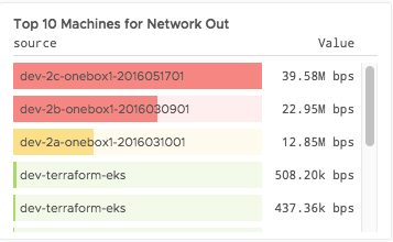
Top or Bottom Time Series
If you’re interested in, for example, the top 3 time series or the bottom 3 time series, evaluated at the current time, use the topk() and bottomk() functions.
topk(3,(ts(~sample.network.bytes.sent, source="app-10")))
bottomk(3,(ts(~sample.network.bytes.sent, source="app-10")))
You can use the topk chart to visualize the top series.
Rate of Change
To enable comparison of an expression with its own past behavior. use lag(). In effect, lag() timeshifts an expression’s data points by a specified time period.
The following example compares the bytes sent with the bytes sent 15 minutes ago:
(ts(~sample.network.bytes.sent, env="dev"))/lag(15m, (ts(~sample.network.bytes.sent, env="dev")))
Queries for Standard Deviation and IQR
We support Anomaly Detection for automatic anomaly detection. You can instead perform anomaly detection with functions and statistical functions. This page gives some examples.
Standard Deviation from Self
Display the number of standard deviations that each series varies from its historic self, that is, standard deviation from the mean, like this:
(ts(~sample.network.bytes.sent, source="app-10"))
- mavg(5d, (ts(~sample.network.bytes.sent, source="app-10")))
/ sqrt(mvar(5d, (ts(~sample.network.bytes.sent, source="app-10"))))
Standard Deviation from All Series
Displays the number of standard deviations from the group of series. (Standard deviation from the mean).
(ts(~sample.network.bytes.sent, env="dev"))
- avg((ts(~sample.network.bytes.sent, env="dev")))
/ sqrt(variance(ts(~sample.network.bytes.sent, env="dev")))
Interquartile Range from Self
The interquartile range (IQR) is the difference between the upper (75th percentile) and lower (25th percentile) quartiles and describes the middle 50% of values when ordered from lowest to highest. The IQR can be a better measure of spread than the range because it is not affected by outliers. Like mean and standard deviation, median and IQR measure the central tendency and spread, but are robust against outliers and non-normal data.
The following example displays the number of IQR’s each series varies from its historic self:
abs(ts(~sample.network.bytes.sent, source="app-10")
- mmedian(5m, (ts(~sample.network.bytes.sent, source="app-10")))
/ (mpercentile(5m, 75, (ts(~sample.network.bytes.sent, source="app-10")))
- mpercentile(5m, 25, (ts(~sample.network.bytes.sent, source="app-10")))))
Interquartile Range from All Series
You can display the IQR of all series, that is, of the population, like this:
abs(ts(~sample.network.bytes.sent, env="dev")
- percentile(50, (ts(~sample.network.bytes.sent, env="dev")))
/ percentile(75, (ts(~sample.network.bytes.sent, env="dev"))
- percentile(25, (ts(~sample.network.bytes.sent, env="dev")))))
Aggregated Result from Multiple Sources by Tag
Assume you have a metric that gives the time in seconds for multiple clusters, for example:
ts(nginx.ingress.controller.ssl.expire.time.seconds)
You can average the results by tag like this:
avg(ts(...), <myrtag)
See Point Tags in Queries for details.
How to Account for Known Downtimes or Events in Uptime Queries
There are times when there are known and expected downtime periods such as maintenance or testing windows. See How to Query for Known Downtimes or Events.
Using exists() With Nested If/Else Statements
With nested if/else statements, the exists() function sometimes exhibits unexpected behavior because of series matching. See Using exists with Nested If/Else Statements for an example and a workaround.