You can combine points from multiple time series using an aggregation function such as sum(), avg(), min(), count(), percentile() etc. An aggregation function returns a series of points whose values are calculated from corresponding points in two or more input time series. VMware Aria Operations for Applications (previously known as Tanzu Observability by Wavefront) supports aggregation with interpolation or without interpolation:
- Standard aggregation functions (e.g.
sum(),avg(), ormax()) first interpolate the points of the underlying set of series, and then apply the aggregation function to the interpolated series. These functions aggregate multiple series down, usually to a single series. - Raw aggregation functions (e.g.
rawsum(),rawavg()) do not interpolate the underlying series before aggregation. - Moving window functions (e.g.
msum(),mavg()andmmax()aggregate series horizontally across a chart by time. They take each individual series and aggregate its own prior behavior across the timeWindow. For example, you can get the maximum value for each series in the specified time window.
In the following video, Clement Pang explains how interpolation works. Note that this video was created in 2018 and some of the information in it might have changed.
Aggregating Data Points That Line Up
The easiest way to see the results of an aggregation function is when all of the input series report their data points at exactly the same time. This causes the points at any given timestamp to all line up. The aggregation function operates on the values in each lineup of points, and returns each result in a point at the corresponding timestamp.
For example, consider the two time series in the following chart. The reporting interval for these series is 1 minute, and the points in these series “line up” at each 1-minute mark on the x-axis. We use a point plot to reveal the correspondences between reported points.

Now we use the sum() function to aggregate these two time series. Each blue point produced by sum() is the result of adding the data values reported by the input series at the same minute.

Aggregating When Data Points Do Not Line Up
In many cases, the set of time series you specify to an aggregation function will have data points that do not “line up” at corresponding moments in time. For example:
- All input series might report data points regularly, but some might report at a longer or shorter interval than the others.
- One input series might report at irregular times that don’t match the reporting times of any other input series.
- One otherwise regular input series might have gaps due to reporting interruptions (e.g., intermittent server or network downtime) which are not experienced by the other input series.
The query engine provides two kinds of aggregation functions for handling this situation:
- Standard aggregation functions fill in the gaps in each input series by interpolating values, and therefore operate on interpolated values as well as actual reported data points.
- Raw aggregation functions do not interpolate the underlying series before aggregation, but rather operate only on actual reported data points.
Standard Aggregation Functions (Interpolation)
Standard aggregation functions fill in the gaps in each input series by interpolating values.
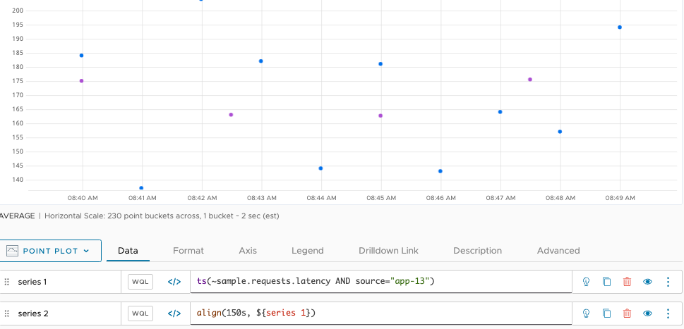
For example, let’s start with a pair of series with reporting intervals that do not line up. In the following chart, series 1 reports once a minute. We can use align() to have series 2 report only every 150 seconds (2.5 minutes). Both series have data points aligned at the 5 minute marks, but the points in between are not aligned.
Now we use the sum() function (a standard aggregation function) to aggregate these two time series. In the following chart, we see that sum() produces a result for every moment in time that a data point is reported by at least one input series. Whenever both series report a data point at the same time (at each 5 minute mark), sum() returns a data point whose value is the sum of both reported points.
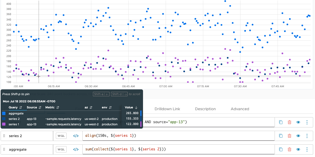
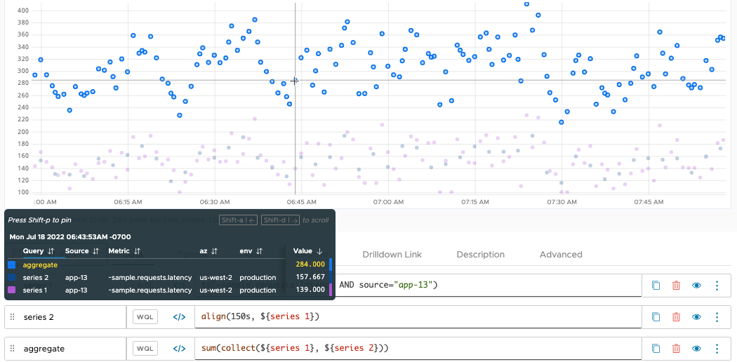
The result at 6:43 is more interesting. At this moment in time, only series 1 reports a point, but sum() returns the value 284.00. sum() produces the return value by adding the actual value of series 1 to an interpolated value from series 2. Interpolation inserts an implicit point into series 2 at 6:43, and assigns an estimated value to that point based on the values of the actual, reported points. sum() uses the estimated value (in this case, 139) to calculate the value returned at 6:43.
Requirements for Interpolation
The query engine interpolates a value into an input time series only under the following circumstances:
-
When at least one other input time series reports a real data value at the same moment in time. In our example, no values are interpolated at, say, 4:26:30, because neither input series reports a point at that time.
-
When the time series has an actual reported value on either side of it. Sometimes this cannot occur, for example, when a new data point has not been reported yet at the right edge of a live-view chart. In this case, the query engine inserts implicit points wherever needed, and assigns the last known reported value in the time series to those implicit points. (The last known reported value must be reported within the last 15% of the query time in the chart window.)
Raw Aggregation Functions (No Interpolation)
You can use raw aggregation functions instead of standard aggregation functions if you want the results to be based on actual reported values, without any interpolated values. For example, you might use raw aggregation results as a way of detecting when one or more input time series fail to report a value.
Let’s see how the raw aggregation function rawsum() treats the two sample time series from the previous section. The following chart shows that rawsum(), like sum(), produces a result for every moment in time that a data point is reported by at least one input series.
Unlike sum(), rawsum() produces its results by adding up just the actual values at each reporting moment. At 4:26, for example, rawsum() returns 164.00, which is the only value reported at this time. No values from series 2 are present at that time, and none are interpolated.

Whenever both series report a data point at the same time (for example, 4:25), rawsum() returns a data point whose value is the sum of both reported points (169.05 + 162 = 331.05).
Filtering the Aggregation Input
You use an expression to describe the set of time series to be aggregated. When using a ts() expression, you can include filters to narrow the set. For example, if multiple sources are reporting the metric ~sample.cpu.loadavg.1m:
sum(ts(~sample.cpu.loadavg.1m))shows the sum of the values reported for the metric from all sources.sum(ts(~sample.cpu.loadavg.1m, source=app-1*))shows the sum of the values reported for the metric, but only from sources that matchapp-1*.sum(ts(~sample.cpu.loadavg.1m, source=app-1*, env=prod))further filters the input series to those with the point tagenv=prod.
Grouping the Aggregation Results
Each aggregation function accepts a group by parameter that allows you to subdivide the input time series into groups, and request separate aggregates for each group.
For grouping, we support:
- The implicit
group byparameter after a comma, discussed here. - An explicit
byparameter - An explicit
withoutparameter.
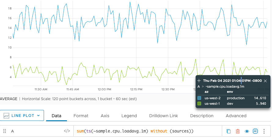
A chart displays a separate line for each group when you use a group by parameter with an aggregation function. For example, assume your environment uses an az point tag to group by availability zone. You call:
sum(ts(~sample.cpu.loadavg.1m), az)
The call groups the result of the call to sum() into two time series, one for each availability zone.
| 'Group By' Parameter | Description | Example |
|---|---|---|
| metrics | Group the series with the same metric name. | sum(ts(cpu.loadavg.1m), metrics) |
| sources | Group the series that are reported from the same source. | sum(ts(cpu.loadavg.1m), sources) |
| sourceTags | Group the series that are reported from sources with the same source tag names. A source tag is valid only if it is explicitly specified in the ts() expression. | sum(ts(cpu.loadavg.1m, tag=prod or tag=db),sourceTags) |
| pointTags | Group the series by all available point tag keys. | sum(ts(cpu.loadavg.1m), pointTags) |
| <pointTagKey> | Group the series with common values for a particular point tag key. Specify the point tag key by name, such as region. |
sum(ts(cpu.loadavg.1m), region) |
Grouping with by or without
You can the following grouping keywords in a query:
- The
bykeyword has the same result as the comma in a query. The following two queries are equivalent:sum(ts(~sample.cpu.loadavg.1m), az, sources) sum(ts(~sample.cpu.loadavg.1m) by (az, sources)) - The
withoutkeyword allows you to group all possible group parameters except for those listed. The following example groups all available grouping parameters except for sources and source tags. In this case, that means grouping by the two point tag keysazandenv.
A Closer Look at Grouping with sourceTags
The sourceTags parameter behaves a little differently from the other grouping parameters. sourceTags produces a subgroup that corresponds to each source tag that is explicitly specified in the ts() expression. No other source tags are taken into account.
For example, suppose you added 3 source tags (prod, db, and highPriority) to the metric cpu.loadavg.1m, and now you want to use the sourceTags parameter with sum() to return subtotals based on the source tags.
-
The following query returns only 2 subtotals - one for the group with the source tag
prodand one for the group with the source tagdb:sum(ts(cpu.loadavg.1m, tag=prod or tag=db),sourceTags) -
The following query returns 3 subtotals, one for each source tag:
sum(ts(cpu.loadavg.1m, tag=prod or tag=db or tag=highPriority),sourceTags)
In contrast, a group by parameter like pointTags produces a separate aggregate corresponding to every point tag that is associated with the specified time series, even if the ts() expression does not explicitly specify any point tags as filters.
Aggregation Example
The chart below represents 3 unique series reporting latency data. The sections with dashed lines represent gaps where no data is reported.

The series report data like this:
- Two of the reporting series have gaps of missing data between 9:15a and 9:21a.
- All three reporting series have gaps of missing data between 9:27a and 9:30a
- One reporting series has a gap of missing data between 9:36a and 9:42a.
The following chart shows what happens when we apply sum() (orange line) and rawsum() (blue line) to the three time series.
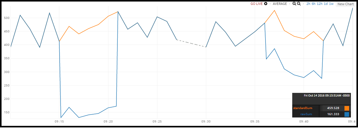
The lines are different because interpolation occurs with the standard aggregation function (sum()), but not with the raw aggregation function (rawsum()).
Example: Standard Aggregation Function
When there is at least 1 true data value reported at a given interval, standard aggregation functions interpolate data values before executing the aggregation.
The data values in the charts above are typically reported once a minute. In the chart that shows the 3 time series, we see that:
- Between 9:15a and 9:21a, the orange series reports once a minute, on the minute, while the other two series do not. Because the orange series reports at least 1 true data value during this time, the query engine interpolates the values for the blue and green series before calculating the
sum()value. - Between 9:36a and 9:42a the green and orange series report data values every minute, but the blue series does not. The query engine does interpolation before aggregation.
Example: Raw Aggregation Function
Raw aggregation functions on the other hand calculate aggregates based on actual reported values (no interpolation).
- Between 9:15a and 9:21a, the
rawsum()values are approximately 1/3 of thesum()values (1 of 3 series reported values) - Between 9:36a and 9:42a, the
rawsum()values are approximately 2/3 of thesum()value (2 of 3 series reported values).
Note that the gap between 9:27a and 9:30a is exactly the same regardless of which aggregation function type we use. None of the series included in the aggregation reported a data value during this time. As a result, the standard aggregation function does not apply interpolated values during this gap, and the result of aggregation looks the same for sum() and rawsum().
The behavior differences between standard and raw apply to all aggregation functions (sum, avg, min, max, count, variance, percentile).
Aggregation Best Practice – When to Use Raw or Aggregated Data
Your use case and data shape determines whether running queries over raw data or over aggregated data makes more sense.
- Use aggregated data if you want quick and precise results for all points in time in which at least one time series reported.
- Use raw data if you aggregate over a large search space (many time series, long time). When the system has to perform interpolation (see above) over a large search space, query performance can suffer.
- As a compromise, consider calling
align()before applying raw aggregation functions, for example,rawsum(align(1m, ts("my_data")))
Here are some details:
What’s Your Data Shape?
Interpolation requires additional resources. Using a non-raw aggregation function on several thousand time series might affect query performance – and if you’re looking at several weeks or months of data, you’ll need even more resources. For those cases, consider using raw aggregation, which comes at the cost of slightly less precision.
Are Skipped Values Common in the Data You’re Analyzing?
Consider whether your time series have natural gaps and what you want to do for those cases. For example, suppose you want to aggregate the number of errors reported across multiple time series. Does the time series report 0 at regular intervals when no errors occur or skip the reporting interval?
- If the time series reports 0 when there’s no value, you don’t need interpolation and can safely use the raw aggregation function.
- If the time series skips the reporting interval, consider whether you want interpolation, that is, “pretend” there is a value even though there is no value – or possibly change the data sources to report 0 is a solution.
Are Reporting Intervals Staggered?
If reporting intervals are staggered, non-raw aggregation (and interpolation) can give you quick value.
For example, suppose you’re evaluating 10 time series over a 1 hour window. Each time series reports once per minute, but they don’t report at the same time (align). By using a non-raw aggregation function you can get interpolation and a fast result.
If, in that same scenario, you’re evaluating 1000 time series over a 1 week time window, a large data set results and interpolation might impact performance. For that case, you can use align() together with a raw aggregation function to get the benefit of aligned data without the performance hit of interpolation, for example:
rawavg(align(1m, ts("my_data")))
Learn More!
The KB article When to use raw vs. non-raw aggregation gives additional detail.